
Attitude Estimation Explained: Rotation Matrices, Euler angles, Quaternions, and Sensor Fusion
May 25, 2026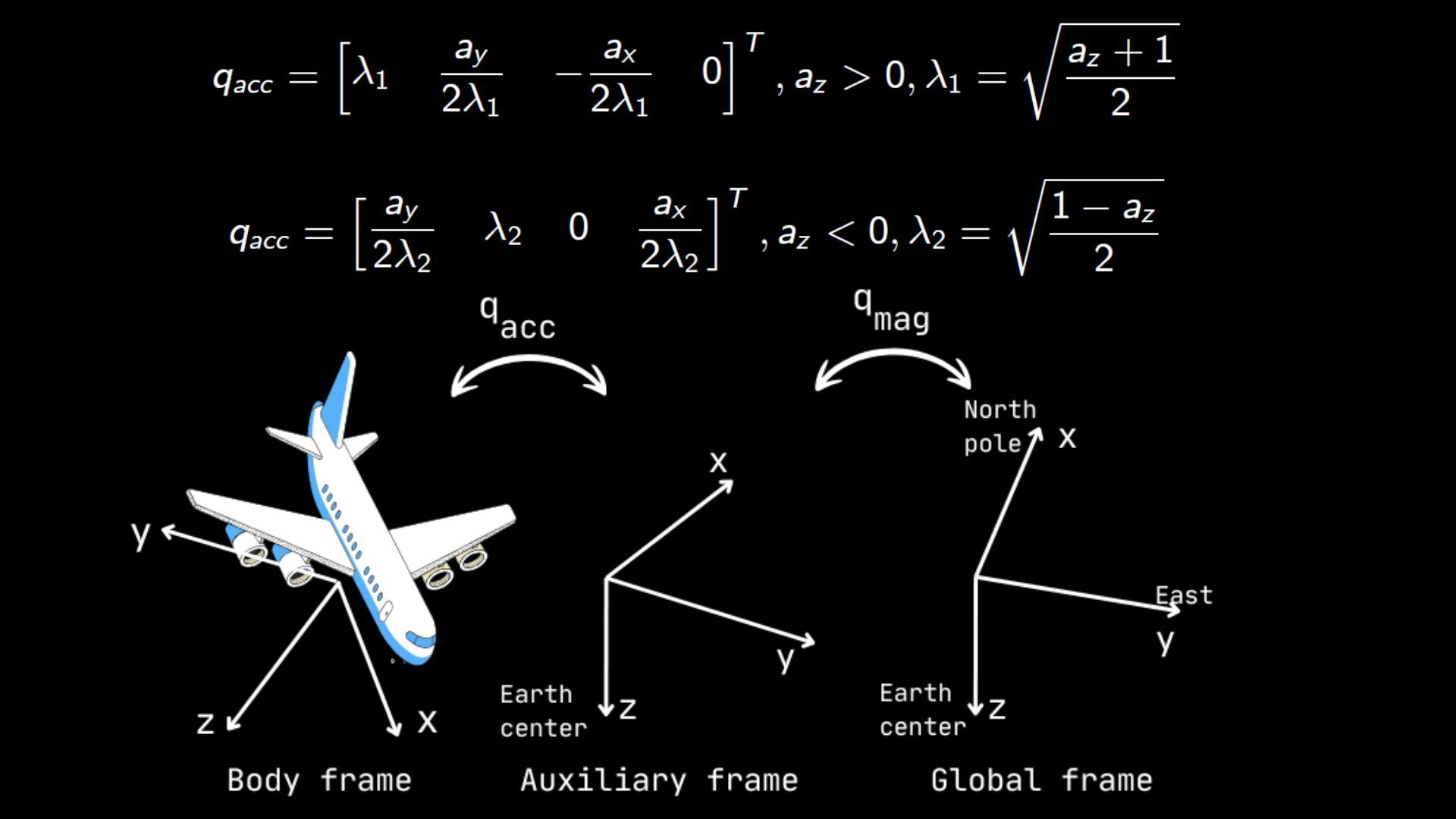
IMU Attitude Estimation
Complementary Filter · Madgwick Filter · Extended Kalman Filter
How does a drone know which way it is pointing? How does a phone screen flip when you tilt it? The answer is attitude estimation — the art of computing orientation from the raw measurements of an inertial measurement unit (IMU). An IMU combines a three-axis accelerometer, a three-axis gyroscope, and optionally a three-axis magnetometer. Each sensor is useful on its own, yet each is also fundamentally limited: the accelerometer is noisy during motion, the gyroscope drifts over time, and the magnetometer is disturbed by nearby metal. Getting accurate, stable orientation requires fusing all three, and that fusion is the subject of this article.
We build up the theory from first principles. We begin with rotation matrices — the mathematical backbone of any orientation representation — and derive how the three elementary rotations (yaw ψ, pitch θ, roll φ) compose into a single rotation matrix $R_\text{total}$. We then show how each sensor constrains that matrix: the accelerometer fixes roll and pitch using the gravity vector; the magnetometer fixes yaw using the Earth's magnetic field; and the gyroscope propagates orientation forward in time using the Euler kinematic equations. With that foundation in place, we cover three fusion algorithms of increasing sophistication:
- Complementary filter — a single tuning parameter α blends the low-noise gyroscope prediction with the drift-free accelerometer/magnetometer correction, in both Euler-angle and quaternion form.
- Madgwick filter — a gradient-descent algorithm that minimizes the error between the predicted and measured field vectors, operating entirely in quaternion space for robustness against gimbal lock.
- Extended Kalman Filter (EKF) — the probabilistic gold standard. The quaternion state is propagated by the gyroscope (prediction phase) and corrected by the accelerometer and magnetometer (update phase) using a full covariance matrix and Jacobian linearization.
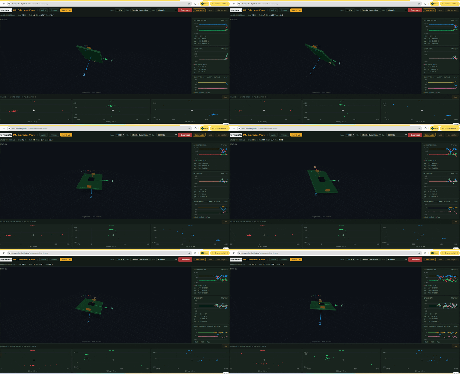
All three algorithms can be explored interactively with the open-source IMU Orientation Viewer. Connect any compatible hardware over USB serial — or click Demo Mode to run a simulated IMU with realistic gyro drift and noise — and watch your board's roll, pitch, and yaw update live in 3D while the charts show the raw sensor data underneath. Switching between filters is a single click, making it easy to feel the difference between complementary smoothness, Madgwick responsiveness, and EKF accuracy.
1. What is Attitude?
Imagine strapping an electronic board to a drone. As the drone flies, the board tilts, rotates, and spins. At any given moment we want to know exactly how the board is oriented — not where it is in space, but which way it is pointing. This orientation is called attitude.
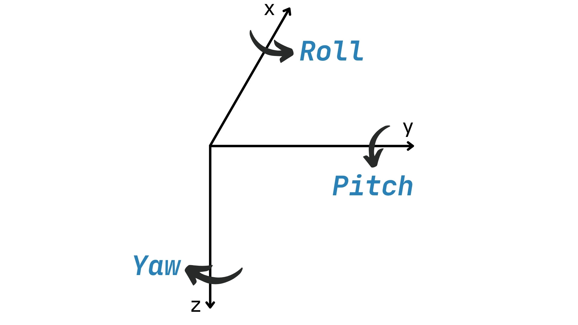
Attitude is described by three angles, one for each axis of rotation:
- Roll (φ) — rotation around the forward axis. Think of a plane banking left or right, or a ship rolling in waves.
- Pitch (θ) — rotation around the side-to-side axis. Think of the nose of an aircraft pointing up or down during climb and descent.
- Yaw (ψ) — rotation around the vertical axis. Think of a car steering left or right, or a compass bearing.
These three angles together are called Euler angles. They are intuitive and easy to visualize, but they have a hidden mathematical problem called gimbal lock, which we explain in Section 9.
2. Two Reference Frames
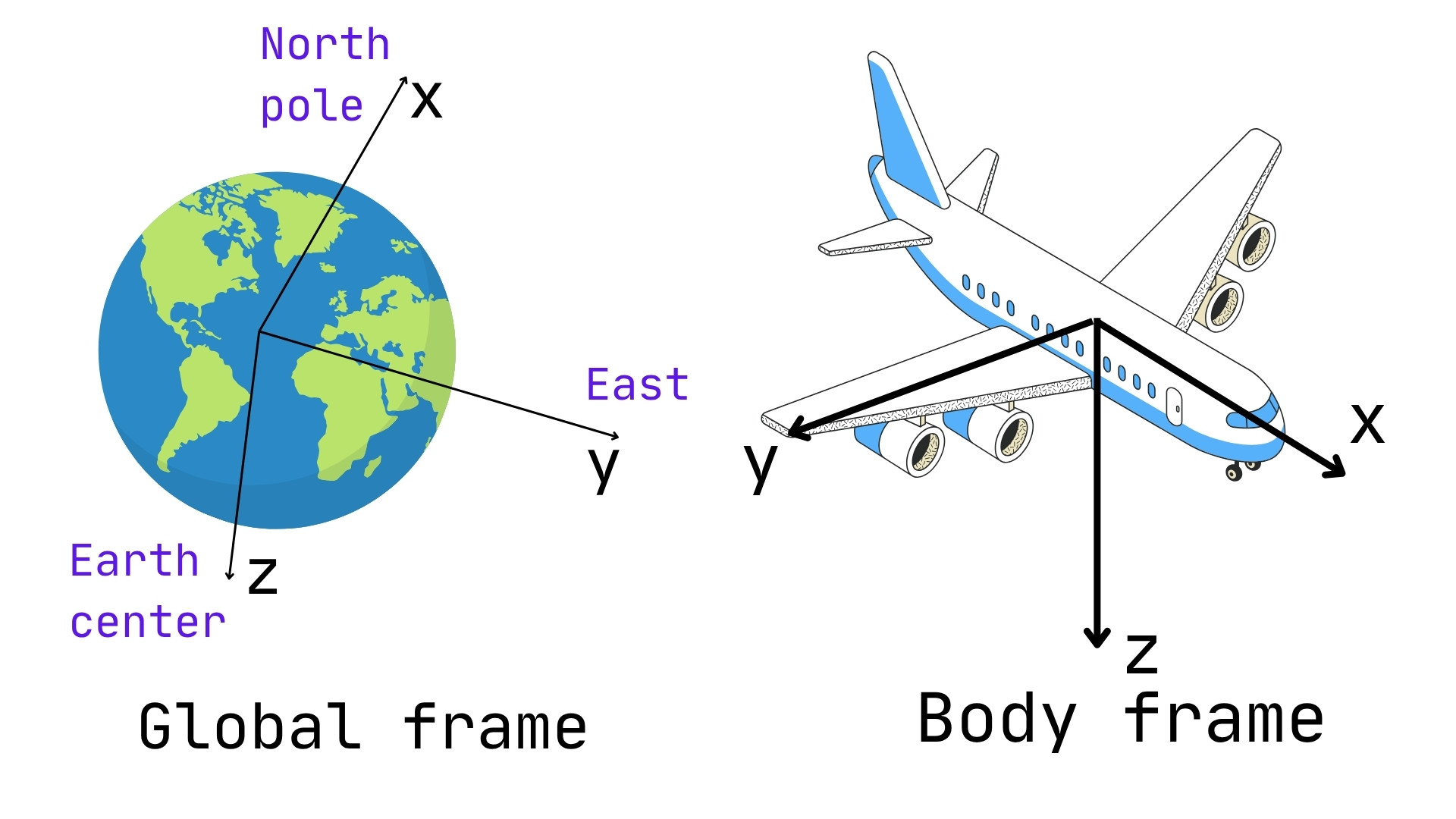
To measure angles, we always need to ask: angles relative to what? In attitude estimation we work with two coordinate systems at the same time.
The Global Frame — fixed to the Earth
The global frame does not move. We use the North-East-Down (NED) convention:
- $X_G$ points North
- $Y_G$ points East
- $Z_G$ points down toward the center of the Earth
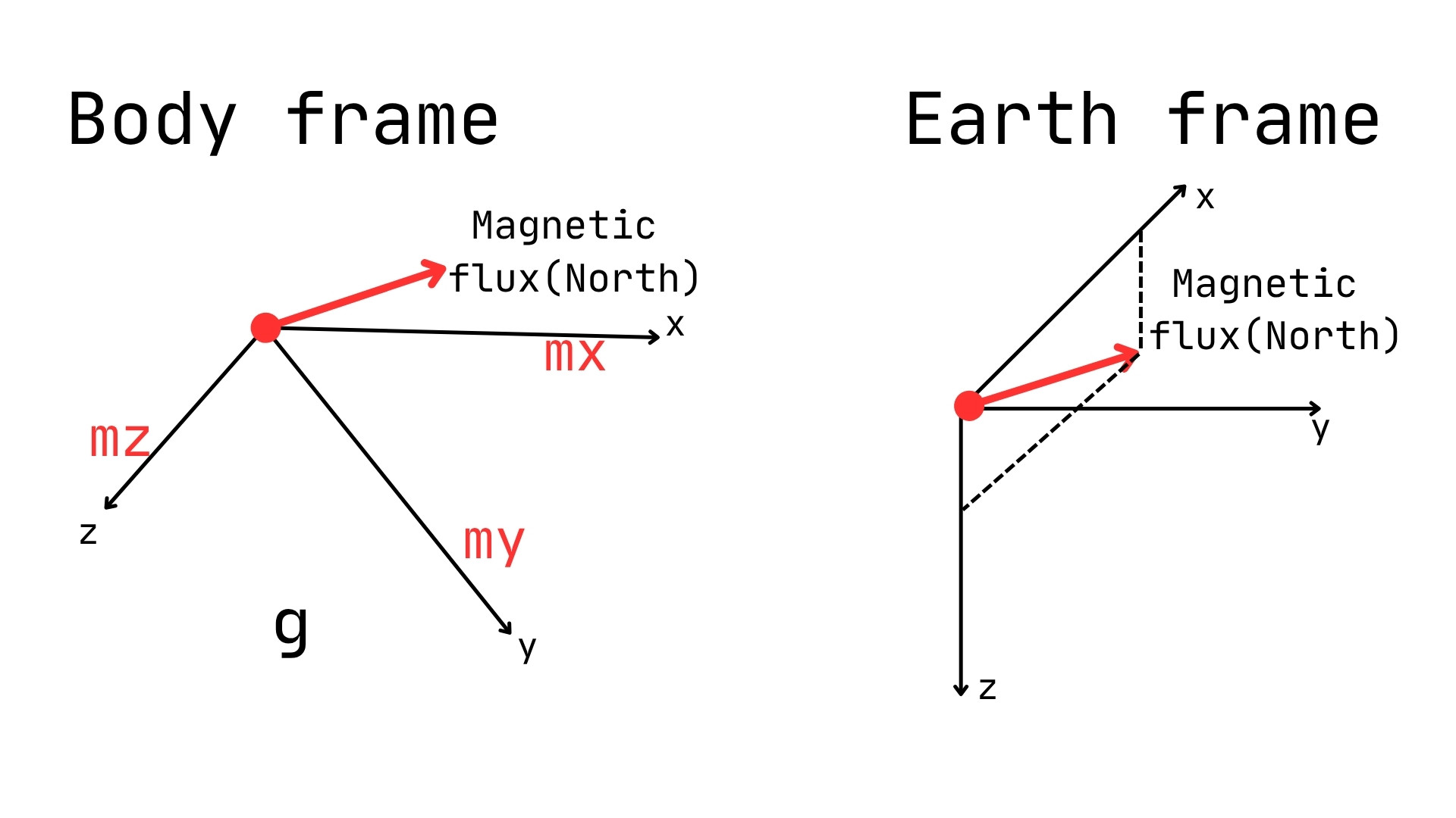
Gravity normalized to 1 is $\mathbf{g} = [0,\; 0,\; 1]^\top$. The Earth's magnetic field has a component $M_x$ pointing North and a component $M_z$ pointing down.
The Body Frame — attached to the sensor
- $X_B$ points forward (out the nose)
- $Y_B$ points right (along the right wing)
- $Z_B$ points down (toward the belly)
Every IMU sensor reports measurements in the body frame. Attitude estimation is the problem of finding the rotation that relates the body frame to the global frame.
3. Rotation Matrices
A rotation matrix transforms a vector from one coordinate frame to another. Every other orientation representation — Euler angles, quaternions — connects back to rotation matrices.
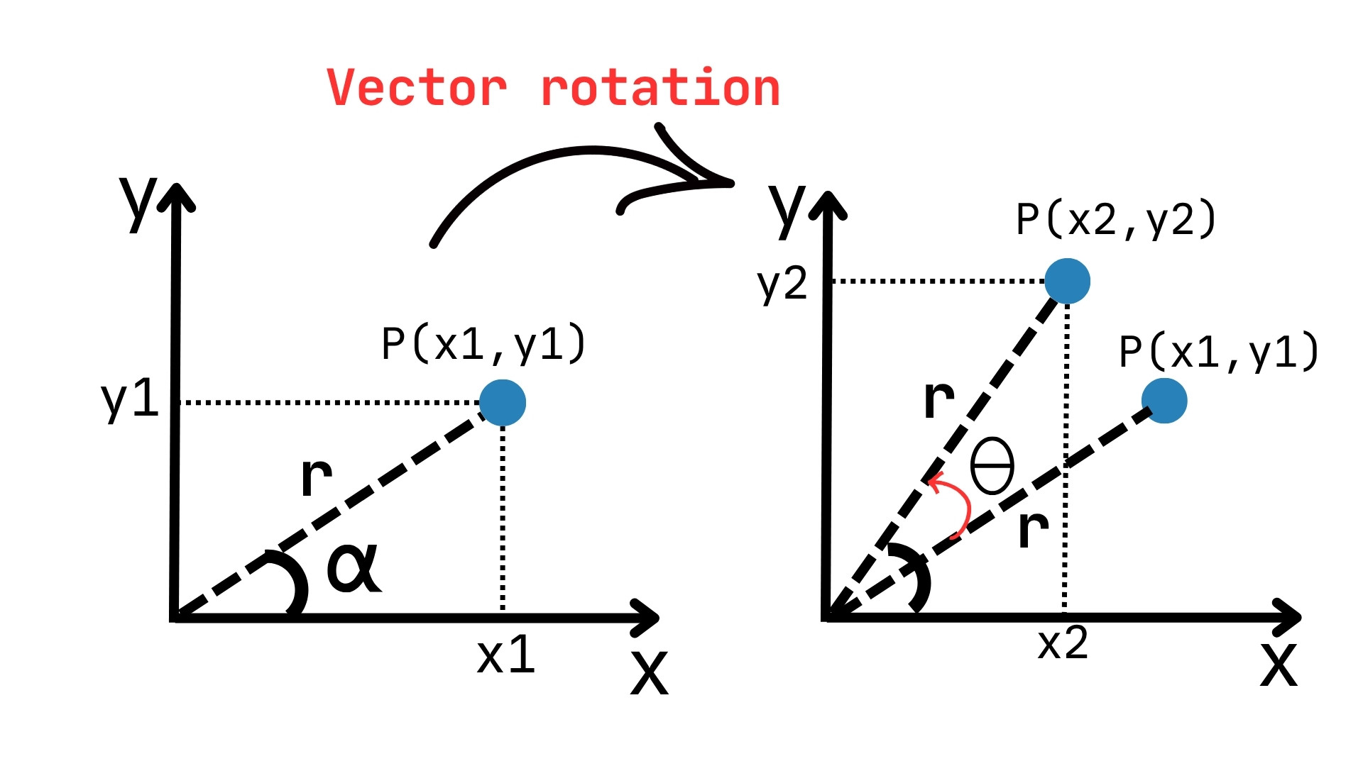
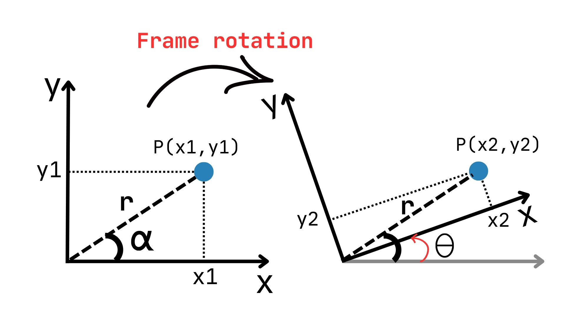
2D Rotation: Two Very Different Questions
Vector rotation — rotate the vector, keep the frame fixed:
Frame rotation — keep the vector, express in a rotated frame:
Frame rotation is the transpose of vector rotation. In IMU work we always use frame rotation to express the global gravity vector in body-frame coordinates.
3D Rotation: The ZYX (Aircraft) Sequence
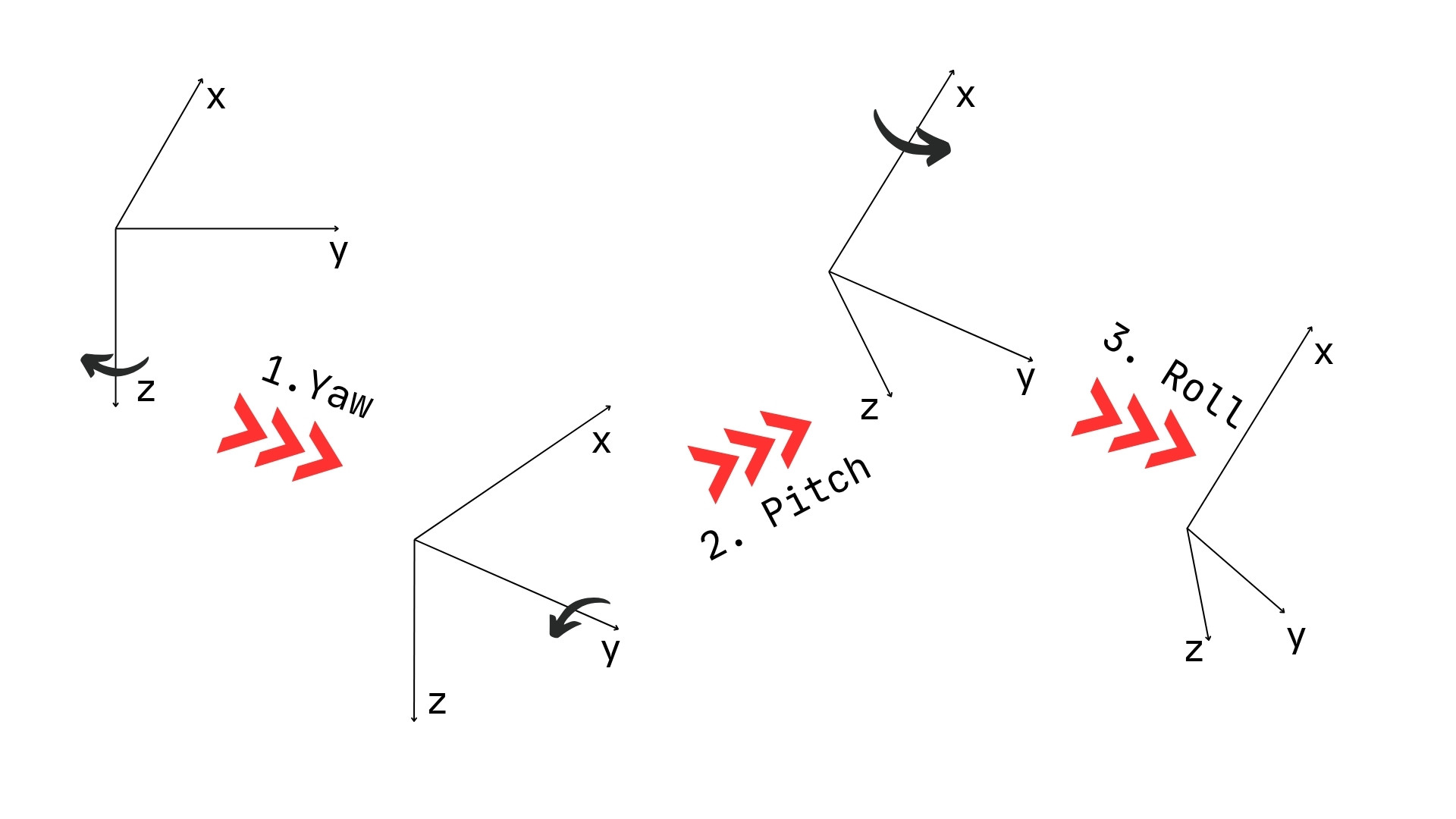
We apply three rotations in sequence — first yaw ($\psi$) around Z, then pitch ($\theta$) around the new Y, then roll ($\phi$) around the new X.
The complete rotation from global to body frame:
Multiplying out (shorthand $c = \cos$, $s = \sin$):
This single $3\times 3$ matrix captures the body's entire orientation. It is orthogonal: $R_\text{total}^{-1} = R_\text{total}^\top$.
4. Accelerometer → Roll and Pitch
An accelerometer measures specific force — at rest, it feels gravity rotated into the body frame:
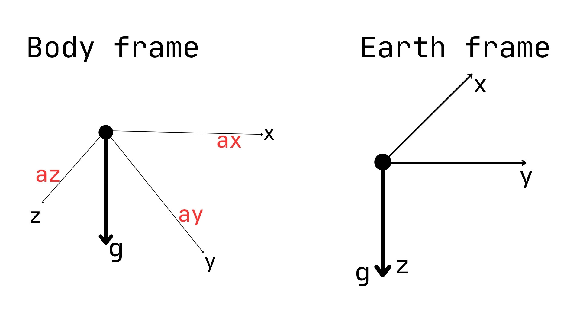
Reading the third column of $R_\text{total}$ gives:
Inverting gives roll and pitch directly:
Why atan2 instead of arctan? The standard arctan only returns $-90°$ to $+90°$. The two-argument form atan2(y, x) uses the signs of both inputs to cover the full $-180°$ to $+180°$ range — essential for roll, which can swing all the way around.
Yaw is absent from equations 12–14: rotating the board about the vertical axis does not change the accelerometer's readings. We need the magnetometer for yaw.
5. Magnetometer → Yaw
The magnetometer reads the Earth's magnetic field rotated into the body frame:
Expanding and solving for $\psi$ using the already-known roll and pitch gives the tilt-compensated heading formula:
Tilt compensation is critical: a tilted magnetometer without it gives the wrong heading. Eq. 23 accounts for the tilt using the known roll and pitch.
6. Gyroscope → Euler Angle Rates
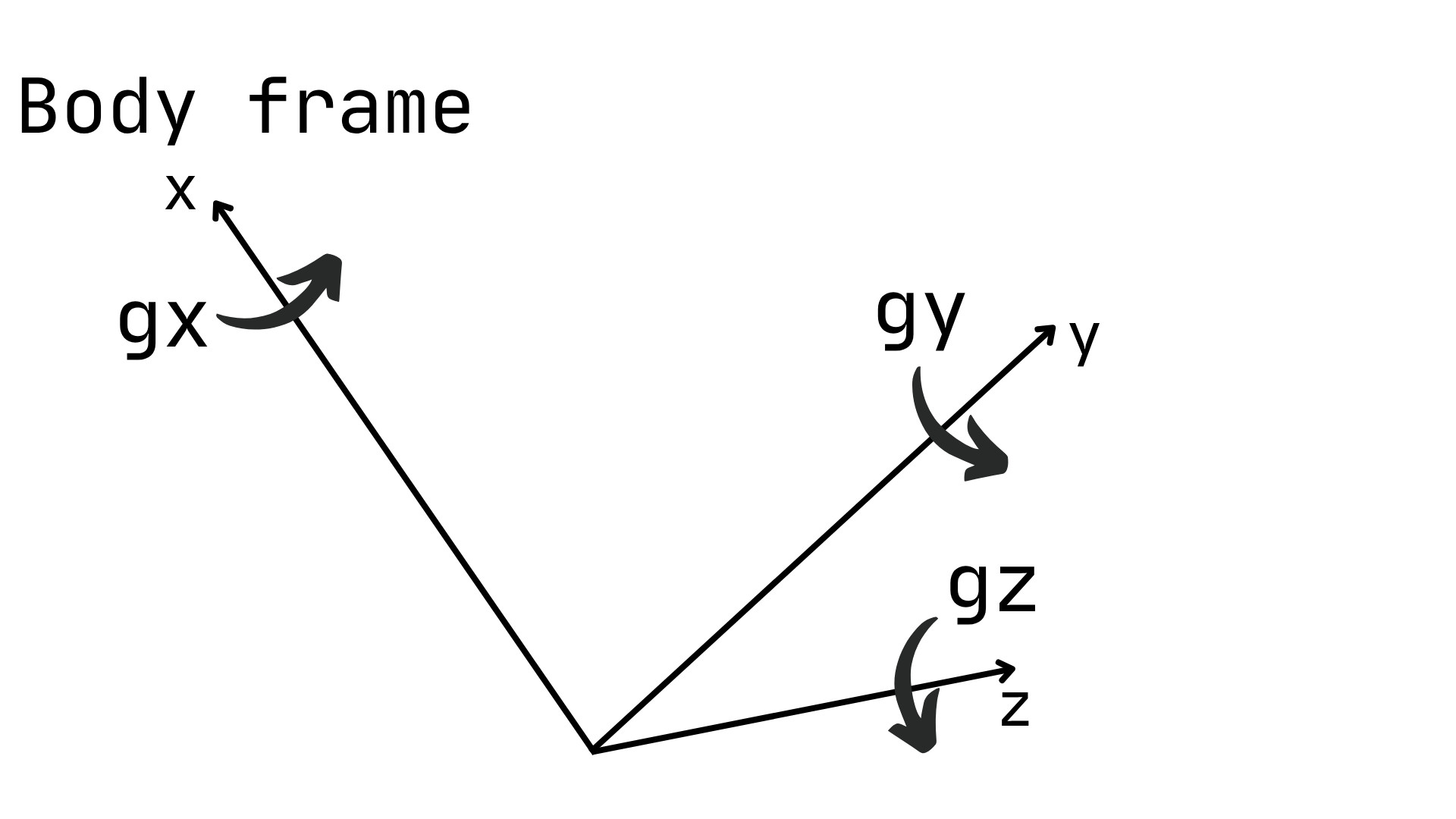
The gyroscope measures body-frame angular rates $[p,\; q,\; r]^\top$ (rad/s). These are not the same as Euler angle rates because roll, pitch, and yaw axes move as the body rotates. The transformation is:
Inverting gives Euler angle rates from the gyro:
Integrate over $\Delta t$ to get new angles:
This works well short-term, but tiny integration errors accumulate — the estimate drifts over time. This is the gyro's fundamental weakness.
7. The Fundamental Problem: Noise vs. Drift
We now have two independent ways to estimate attitude:
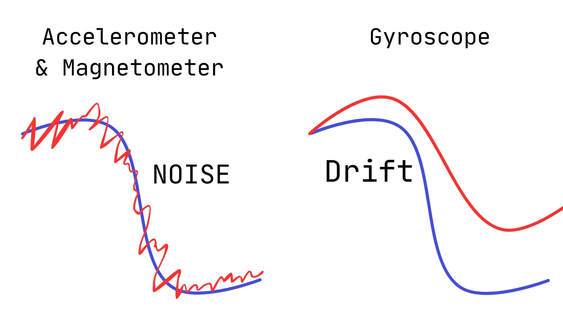
- Accelerometer + Magnetometer: gives absolute angles anchored to physical references — accurate long-term, but noisy (vibration and linear acceleration corrupt the reading).
- Gyroscope: gives smooth, fast angles — but drifts over time due to accumulated integration error.
The accelerometer is like someone who always knows which way is down but gets confused by bumps. The gyroscope is like someone who remembers every turn but slowly loses track of where they started. We must fuse both signals. All three algorithms solve this same problem in different ways.
8. Algorithm 1 — Complementary Filter
The complementary filter is the simplest sensor fusion method. The gyroscope provides fast high-frequency components; the acc/mag provides the stable long-term low-frequency anchor. Together they cover the full frequency range.
The Formula
With $\alpha = 0.98$: 98% smooth gyro + 2% absolute correction. The correction stops drift without making the output noisy. Equivalently:
Steps to Implement
- Receive raw IMU data. Normalize the accelerometer to unit length.
- Compute roll $\phi$ and pitch $\theta$ from the accelerometer (eqs. 15, 16).
- Compute yaw $\psi$ from the tilt-compensated magnetometer (eq. 23).
- Compute new Euler angles by integrating the gyroscope (eqs. 26, 27).
- Blend both estimates using eq. 28 with your chosen $\alpha$.
Choosing α
| α | Behavior | Best for |
|---|---|---|
| 0.99 | Very strong gyro trust. Very slow drift correction. | Slow dynamics, low vibration |
| 0.95 – 0.98 | Balanced. Good default starting point. | General use |
| 0.85 – 0.90 | Fast acc/mag correction. Noisy output. | High vibration, short bursts |
9. Gimbal Lock and Why We Need Quaternions
The inversion matrix in eq. 26 contains $\sin\phi/\cos\theta$ and $\cos\phi/\cos\theta$. When pitch reaches $\theta = \pm 90°$, we have $\cos\theta = 0$ — division by zero. The matrix becomes singular.
This is gimbal lock: rolling and yawing produce identical rotations — two degrees of freedom collapse into one. There is no algebraic fix; it is a fundamental limitation of Euler angles.
The solution is quaternions: four-number orientation representation with no equivalent singularity, valid at all orientations.
10. Quaternion Mathematics
A quaternion is a four-dimensional extension of complex numbers (Hamilton, 1843):
In code: $q = [q_0, q_1, q_2, q_3]^\top$ with $q_0$ as the scalar. The imaginary units obey Hamilton's rules:
Quaternion multiplication is not commutative — order matters, just as it does with 3D rotations.
Key Properties
- Norm: $|q| = \sqrt{q_0^2 + q_1^2 + q_2^2 + q_3^2}$
- Unit quaternion: $|q| = 1$ — always renormalize after each update
- Conjugate: $q^* = [q_0,\; -q_1,\; -q_2,\; -q_3]^\top$
- Inverse (unit): $q^{-1} = q^*$
Quaternion Product (Matrix Form)
Rotating Vectors
- Vector rotation: $p' = q\, p\, q^{-1}$
- Frame rotation: $p' = q^{-1}\, p\, q$
The equivalent $3\times 3$ rotation matrix:
11. Accelerometer and Magnetometer as Quaternions
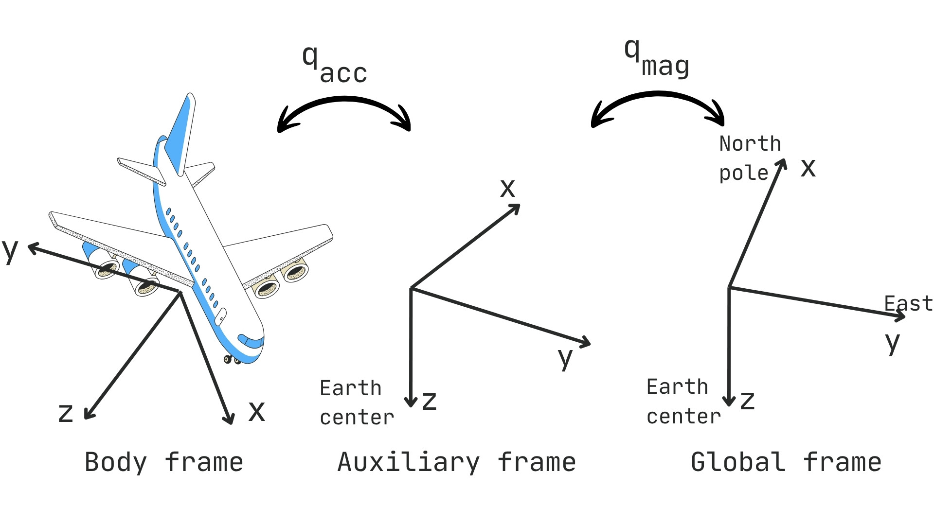
We can compute a quaternion directly from sensor readings, bypassing Euler angles and all trigonometric singularities.
Step 1 — Accelerometer → qacc
When $a_z > 0$, let $\lambda_1 = \sqrt{(a_z + 1)/2}$:
When $a_z < 0$, let $\lambda_2 = \sqrt{(1 - a_z)/2}$:
Step 2 — Magnetometer → qmag
Rotate the mag reading into the auxiliary frame using $q_\text{acc}$:
When $l_x > 0$:
When $l_x < 0$:
Step 3 — Final Quaternion
Gyroscope Quaternion Update
Normalize $q_\text{new}$ after each step. The quaternion complementary filter blends $q_\text{gyro}$ and $q_\text{acc,mag}$ directly; flip the sign of $q_\text{acc,mag}$ if their dot product is negative (to take the short arc), then normalize.
12. Algorithm 2 — Madgwick Filter
The Madgwick filter (Sebastian Madgwick, 2010) works entirely in quaternion space and uses gradient descent to correct the gyro-integrated quaternion. It is more accurate than the complementary filter, handles gimbal lock automatically, and is light enough for small microcontrollers.
Objective Function
Gradient Descent Correction
Full Update
Normalize $q_\text{new}$. The magnetometer adds a second objective function using an Earth field reference $[b_x, 0, b_z]^\top$ computed from the current quaternion — this automatically adapts to local magnetic conditions.
Choosing β
| β | Effect |
|---|---|
| 0.01 – 0.05 | Very smooth. Drift corrects slowly. |
| 0.1 | Good default — balanced accuracy and smoothness. |
| 0.3 – 0.5 | Fast correction, noticeably noisy output. |
13. Algorithm 3 — Extended Kalman Filter
The EKF computes the optimal blending weights automatically at every step based on how uncertain the current estimate is, tracking both the orientation and its uncertainty simultaneously.
State and Uncertainty
State: $q = [q_0, q_1, q_2, q_3]^\top$. Uncertainty: $4\times 4$ covariance matrix $\Sigma$. Large $\Sigma$ = uncertain; small $\Sigma$ = confident.
Phase 1 — Prediction (Gyroscope)
After prediction, $\Sigma$ grows — gyroscope noise added uncertainty. $M$ maps gyro noise (rad/s) into quaternion space.
Measurement Model
Jacobian of the Measurement Model
Phase 2 — Correction (Sensors)
Normalize $q_n$. The Kalman gain adapts automatically: small when sensors are noisy, large when state uncertainty is large.
| Parameter | Meaning | Effect of increasing |
|---|---|---|
| $Q$ | Gyroscope rate noise variance | Trust gyro less, rely more on sensors |
| $R_a$ | Accelerometer noise | Trust acc less, rely more on gyro |
| $R_m$ | Magnetometer noise | Trust mag less |
| $M_x, M_z$ | Local Earth field components | Must match your location for correct yaw |
14. Algorithm Comparison
| Property | Complementary | Madgwick | Extended Kalman Filter |
|---|---|---|---|
| State | Euler angles | Quaternion | Quaternion |
| Gimbal lock | Yes (±90° pitch) | No | No |
| Computational cost | Very low | Medium | High |
| Tuning parameters | $\alpha$ | $\beta$ | $Q,\, R_a,\, R_m,\, M_x,\, M_z$ |
| Magnetometer support | Yes | Yes | Yes |
| Statistically optimal | No | No | Yes (Gaussian noise) |
| Adaptive weights | No | No | Yes (Kalman gain) |
| Best for | Learning, limited MCUs | General embedded systems | High-accuracy applications |
Which filter should you use? Start with the Complementary Filter to verify your sensor pipeline. Switch to Madgwick for better accuracy at low complexity. Use the EKF when you need the best accuracy and can invest in tuning — precision robotics, industrial measurement, or anywhere drift must be provably bounded.